Predicting Home Values: A Full Data Science Project Walkthrough

In this blog post, I've taken you on a comprehensive, step-by-step journey through a real-world data science project: predicting home values in West Roxbury, Boston. I started by defining the core problem and outlining our industry, stakeholders, goals, and the benefits of achieving them. From there, I walked through the crucial stages of data collection, showing how I loaded and prepared the WestRoxbury.csv file. You've seen my approach to data cleaning, where I tackled missing values and standardized column names to ensure our dataset was pristine. Then, we dove deep into data exploration (EDA), visualizing relationships and uncovering insights before moving on to feature engineering to prepare our data for modeling.

1. Problem Definition

• Example: Predict the value of homes in West Roxbury, Boston, MA
• Industry: Real Estate
• Stakeholder: Zillow
• Goal: To become the dominant platform for checking house prices
• Benefits: If the goal is achieved, more realtors will pay Zillow for advertising and hence become the dominant online advertising venue for realtors.

2. Data Collection

Usually, we find this data in databases, or we have to web scrape to get the data, or there might be some API that can have the data we want. We found the city housing data that are used to estimate property values for tax assessment.

In this file WestRoxbury.csv we have the data.

import pandas as pd
import numpy as np
import matplotlib.pyplot as plt
import seaborn as sns
from sklearn.model_selection import train_test_split
from sklearn.linear_model import LinearRegression

let's talk a little bit about the libraries we imported

• pandas: to manipulate the csv file and work with tables
• numpy: to do math operations ig
• matplotlib and seaborn: to visualize data on plots and charts idk why we are using two libraries
• sklearn: we are just importing train_test_split, its purpose is to just split the data to use some of it for testing and the remaining for the training

housing_df = pd.read_csv("WestRoxbury.csv")

we used the pandas library to load the data from the csv file

• Note: df in the name of the variable stands for "data frame"

3. Data Cleaning

print(housing_df)

      TOTAL VALUE    TAX  LOT SQFT   YR BUILT  GROSS AREA   LIVING AREA  \
0            344.2  4330       9965      1880         2436         1352   
1            412.6  5190       6590      1945         3108         1976   
2            330.1  4152       7500      1890         2294         1371   
3            498.6  6272      13773      1957         5032         2608   
4            331.5  4170       5000      1910         2370         1438   
...            ...   ...        ...       ...          ...          ...   
5797         404.8  5092       6762      1938         2594         1714   
5798         407.9  5131       9408      1950         2414         1333   
5799         406.5  5113       7198      1987         2480         1674   
5800         308.7  3883       6890      1946         2000         1000   
5801         447.6  5630       7406      1950         2510         1600   

      FLOORS   ROOMS  BEDROOMS   FULL BATH  HALF BATH  KITCHEN  FIREPLACE  \
0         2.0      6        NaN          1          1        1          0   
1         2.0     10        NaN          2          1        1          0   
2         2.0      8        NaN          1          1        1          0   
3         1.0      9        5.0          1          1        1          1   
4         2.0      7        3.0          2          0        1          0   
...       ...    ...        ...        ...        ...      ...        ...   
5797      2.0      9        3.0          2          1        1          1   
5798      2.0      6        3.0          1          1        1          1   
5799      2.0      7        3.0          1          1        1          1   
5800      1.0      5        2.0          1          0        1          0   
5801      2.0      7        3.0          1          1        1          1   

     REMODEL  
0        NaN  
1     Recent  
2        NaN  
3        NaN  
4        NaN  
...      ...  
5797  Recent  
5798     NaN  
5799     NaN  
5800     NaN  
5801     NaN  

[5802 rows x 14 columns]

we can print the data in the terminal, but there are better ways to do this 🧏

print(housing_df.shape)

(5802, 14)

this prints the (rows_num , coloumn_num)

print(housing_df.columns)

Index(['TOTAL VALUE ', 'TAX', 'LOT SQFT ', 'YR BUILT', 'GROSS AREA ',
       'LIVING AREA', 'FLOORS ', 'ROOMS', 'BEDROOMS ', 'FULL BATH',
       'HALF BATH', 'KITCHEN', 'FIREPLACE', 'REMODEL'],
      dtype='object')
      

this prints the names of the columns to see what the data we are dealing with is

housing_df = housing_df.rename(columns={'BEDROOMS ':'BEDROOMS'})

we have to remove the space from the name of the column. In this case, we renamed it but without the space. We can just use the strip method and it does it automatically. I don't know why we are doing this.

housing_df.columns = [col_name.strip().replace(" ", "_") for col_name in housing_df.columns]

ok now we loop over each column and change to remove the space from the beginning and the end of each thing with the strip method and replacing each space, I mean the ones between the words, with underscore _ with the replace method. We removed the space and replaced it with the _ to get access to the . functions in the future.

We can also write this line in this syntax to be more readable:

new_columns = []
for col_name in housing_df.columns:
    cleaned_name = col_name.strip().replace(' ', '_')
    new_columns.append(cleaned_name)
housing_df.columns = new_columns

housing_df.head()

The head method will show the first 5 rows in the df

housing_df.loc[0:9]

The loc method takes a range and it shows the data from the range you selected.

housing_df.iloc[0:9,1]

0    4330
1    5190
2    4152
3    6272
4    4170
5    4244
6    4521
7    4030
8    4195
Name: TAX, dtype: int64

The iloc method is the same as the loc, but the second parameter is the index of the column.

housing_df.loc[0:9,"ROOMS"]

0     6
1    10
2     8
3     9
4     7
5     6
6     7
7     6
8     5
9     8
Name: ROOMS, dtype: int64

if we add the second parameter, we get the data from the column we want

housing_df["REMODEL"] = housing_df["REMODEL"].fillna("None")

the fillna method we used to replace any NA values with something we want, in this case, None

housing_df.ROOMS.dtype

dtype('int64')

here we are getting the data type of the column, and thats why we renamed the columns to have _ and not space to access the functions like now

housing_df.dtypes

TOTAL_VALUE    float64
TAX              int64
LOT_SQFT         int64
YR_BUILT         int64
GROSS_AREA       int64
LIVING_AREA      int64
FLOORS         float64
ROOMS            int64
BEDROOMS       float64
FULL_BATH        int64
HALF_BATH        int64
KITCHEN          int64
FIREPLACE        int64
REMODEL         object
dtype: object

we can use this to see if the data is categorical or not, like with the REMODEL column, which is categorical

housing_df.loc[0:9,"REMODEL"]

0      None
1    Recent
2      None
3      None
4      None
5       Old
6      None
7      None
8    Recent
9      None
Name: REMODEL, dtype: object

housing_df.REMODEL = housing_df.REMODEL.astype("category")
housing_df.REMODEL.cat.categories

Index(['None', 'Old', 'Recent'], dtype='object')

the value of the REMODEL column is categorical, so we converted it to a categorical type and we can see the categories with the cat.categories method, the .cat is a method that is used to work with categorical data

na_counts = housing_df.isna().sum()
print(na_counts)

TOTAL_VALUE    0
TAX            0
LOT_SQFT       0
YR_BUILT       0
GROSS_AREA     0
LIVING_AREA    0
FLOORS         0
ROOMS          0
BEDROOMS       3
FULL_BATH      0
HALF_BATH      0
KITCHEN        0
FIREPLACE      0
REMODEL        0
dtype: int64

now we can see the number of NA values in each column, as we can see there are NA values in the BEDROOMS column, lets fix that

housing_df.BEDROOMS.count()

np.int64(5799)

the .count method counts the number of non-NA values in a column

medianBedrooms = housing_df.BEDROOMS.median()
housing_df.BEDROOMS = housing_df.BEDROOMS.fillna(medianBedrooms)

we found the median of the BEDROOMS column and we filled the NA values with the median,there are better ways to do this, but this is one of them

4. Data Exploration (EDA)

we preform expletory data analysis (EDA) to understand the data and find patterns and relationships between the data.
from what I've understood we just have to visualize the data, and find relations

pd.pivot_table(housing_df,index=["REMODEL"],values=["TOTAL_VALUE"],aggfunc=[np.mean,np.std])

the pivot_table is a pandas method that takes four parameters

1. the dataframe we want to pivot in this case housing_df
2. the index we want to pivot on in this case REMODEL, which is a categorical column
3. the values we want to pivot on in this case TOTAL_VALUE, which is a numerical column, we can also pivot on more than one column by providing the column names in the list
4. the aggregation function we want to use in this case mean and std, which is the standard deviation

housing_df.describe()

the describe method is a pandas method that returns a summary of the data in the data frame, which includes the count, mean, standard deviation, minimum, maximum, and quartiles

ax = housing_df.TOTAL_VALUE.hist()
ax.set_xlabel("Total Value")
ax.set_ylabel("Count")
plt.show()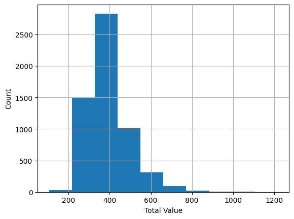

the hist method is used for the columns of the data frame, it returns a histogram of the data, and the set_xlabel and set_ylabel methods are used to set the labels of the x and y axes, and the plt.show method is used to show the plot

housing_df.plot.scatter(x="ROOMS",y="TOTAL_VALUE")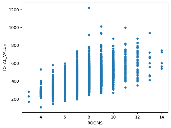

sns.pairplot(housing_df, x_vars=["ROOMS","FLOORS"], y_vars="TOTAL_VALUE", hue="REMODEL",height=5, aspect=.8, kind="reg")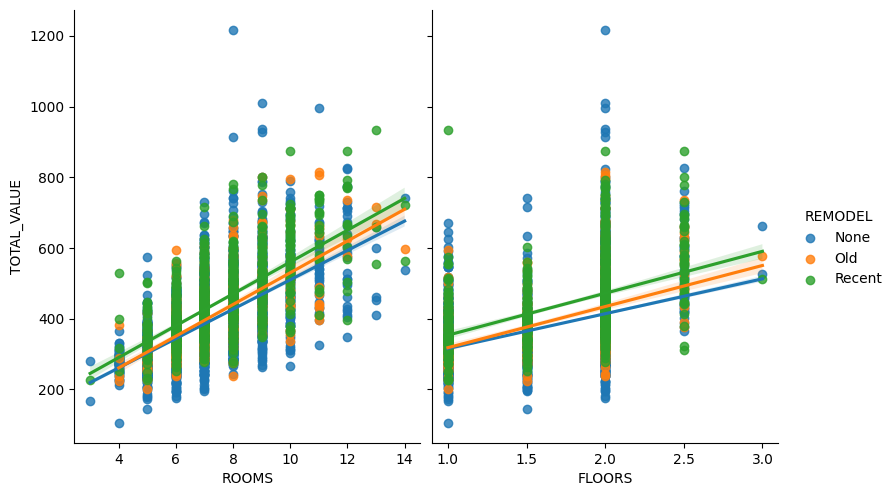

sns.scatterplot(x="LOT_SQFT",y="TOTAL_VALUE",size="FULL_BATH",data=housing_df)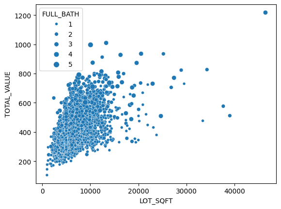

sns.scatterplot(x="LOT_SQFT",y="TOTAL_VALUE",size="FULL_BATH",hue="REMODEL",data=housing_df)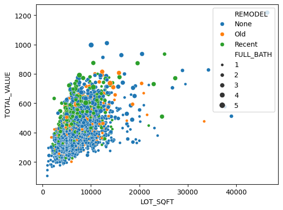

ax = housing_df.boxplot(column="TOTAL_VALUE",by="ROOMS", figsize=(10,10),grid=True)
ax.set_ylabel("Total Value")
plt.suptitle('')
plt.title('')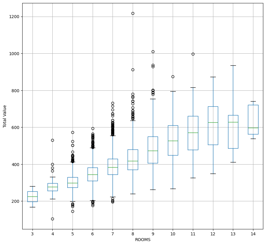

here is Youtube video explaining the above plot

5. Feature Engineering

Create and transform variables (features) that enhance the predictive power of the model. This may involve scaling, encoding categorical variables, or generating new features based on domain knowledge.

housing_df = pd.get_dummies(housing_df,drop_first=True,prefix_sep="_")
housing_df.REMODEL_Old = housing_df.REMODEL_Old.astype("int")
housing_df.REMODEL_Recent = housing_df.REMODEL_Recent.astype("int")
housing_df.head()

any categorical value have to be converted to a binary value, cuz in the regression model i have to have numbers not names and categorys.

we can just take two of the columns and if both of them are zero, we know that the third value is One

6. Modelling

Select suitable algorithms and build predictive or prescriptive models. This involves training machine learning or statistical models using the prepared data, then tuning the models to improve accuracy and reliability.

In this step, dataset is split into:

• Training set (used to build/train multiple models)
• Validation set (used to tune parameters, compare models and select the best model)
• Testing set (held back until final model evaluation to assess the performance of the chosen model).

pay attention to overfitting

excludeColumns = ('TOTAL_VALUE', "TAX")
predectors = [col for col in housing_df.columns if col not in excludeColumns]
X = housing_df[predectors]
y = housing_df["TOTAL_VALUE"]

train_X,valid_X,train_y,valid_y = train_test_split(X,y,test_size=0.7,random_state=1)

1. It excludes the TOTAL_VALUE and TAX columns from the dataset.
2. It assigns the remaining columns to X (features) and TOTAL_VALUE to y (target variable).
3. It splits X and y into training and validation sets using train_test_split, with 70% of the data going into the training set and 30% into the validation set. The split is done randomly, but the randomness is reproducible due to the fixed random_state.

model = LinearRegression()
model.fit(train_X,train_y)

train_predictions = model.predict(train_X)
valid_predictions = model.predict(valid_X)

7. Evaluation

Assess model performance using appropriate metrics (e.g., accuracy, precision, recall, etc.).

train_results = pd.DataFrame({"TOTAL_VALUE":train_y,"predicted":train_predictions, "residuals":train_y-train_predictions})
print(train_results.head())

      TOTAL_VALUE   predicted   residuals
3772        517.5  416.830508  100.669492
3335        325.5  338.979750  -13.479750
2662        419.7  392.672343   27.027657
3546        372.7  364.048194    8.651806
4825        373.8  371.904935    1.895065

This code creates a pandas DataFrame train_results that compares the actual TOTAL_VALUE (train_y) with the predicted values (train_predictions) from a linear regression model. It also calculates the residuals (differences between actual and predicted values). The head() function then prints the first few rows of this DataFrame.

all_residuals = train_y-train_predictions
ax = pd.DataFrame({"residuals":all_residuals}).hist(bins=25)
plt.tight_layout()
plt.show()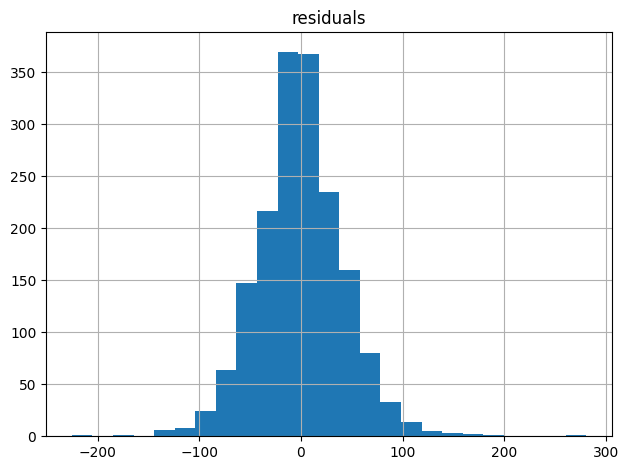

This code calculates the residuals (differences between actual and predicted values) of a linear regression model and visualizes them as a histogram with 25 bins.

We visualize the residuals to check the assumptions of linear regression, specifically:

1. Normality: A histogram of residuals can help verify if the errors are normally distributed, which is an assumption of linear regression.
2. Constant variance: A uniform spread of residuals in the histogram indicates constant variance, another assumption of linear regression.
3. No patterns: A random, scattered pattern in the histogram suggests that the model is capturing the underlying relationships in the data.

By examining the residual histogram, we can identify potential issues with the model, such as non-normality, heteroscedasticity, or non-linearity.

r2= model.score(train_X,train_y)

This code calculates the R-squared (R²) value of the linear regression model on the training data. R² measures the goodness of fit of the model, with higher values indicating better fit (up to a maximum of 1).

but as we said earlier we have to pay attention to overfitting

valid_residuals = valid_y-valid_predictions
ax = pd.DataFrame({"residuals":valid_residuals}).hist(bins=25)
plt.tight_layout()
plt.show()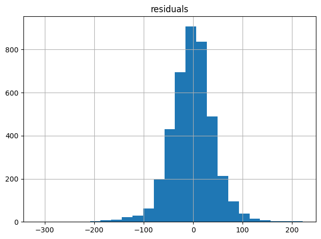

8. Interpretation and Communication

Translate results into actionable insights and communicate findings to stakeholders. This includes explaining model predictions, highlighting key features, and addressing how the findings support the original business problem.

9. Deployment

Implement the model in a real-world environment where it can be used to generate actionable results. This step involves creating a Minimum Viable Product (MVP) by deploying a simplified, essential version of the model to test its effectiveness in solving the problem. During deployment, you may integrate the model with existing systems, develop an API, or set up a dashboard. The MVP allows you to gather initial feedback, monitor
performance, and assess its value to users, providing a foundation for further refinement and scaling based on real-world data and feedback.

new_data = pd.DataFrame({
    'LOT_SQFT': [4200, 6444, 5035],
    'YR_BUILT': [1960, 1940, 1925],
    'GROSS_AREA': [2670, 2886, 3264],
    'LIVING_AREA': [1710, 1474, 1523],
    'FLOORS': [2.0, 1.5, 1.9],
    'ROOMS': [10, 6, 6],
    'BEDROOMS': [4, 3, 2],
    'FULL_BATH': [1, 1, 1],
    'HALF_BATH': [1, 1, 0],
    'KITCHEN': [1, 1, 1],
    'FIREPLACE': [1, 1, 0],
    'REMODEL_Old': [0, 0, 0],
    'REMODEL_Recent': [0, 0, 1],
})

print(new_data)

print('Predictions: ', model.predict(new_data))

   LOT_SQFT  YR_BUILT  GROSS_AREA  LIVING_AREA  FLOORS  ROOMS  BEDROOMS  \
0      4200      1960        2670         1710     2.0     10         4   
1      6444      1940        2886         1474     1.5      6         3   
2      5035      1925        3264         1523     1.9      6         2   

   FULL_BATH  HALF_BATH  KITCHEN  FIREPLACE  REMODEL_Old  REMODEL_Recent  
0          1          1        1          1            0               0  
1          1          1        1          1            0               0  
2          1          0        1          0            0               1  
Predictions:  [384.30511506 377.59257723 385.8679671 ]

and that's it we predicted the values

10. Monitoring and Maintenance

Continuously monitor the model’s performance to ensure it remains accurate over time. Regular updates may be needed as new data becomes available or if the business problem evolves

Conclusion

As we conclude this project, I hope I've clearly illustrated the complete data science lifecycle, from our initial problem definition all the way to model deployment. We've meticulously cleaned and explored our raw data, transforming it into meaningful features, and then built and rigorously evaluated our linear regression model. The successful prediction of new home values at the end, as shown with our new_data DataFrame, truly showcases the tangible outcome of this systematic process. Remember, data science isn't a one-and-done deal; continuous monitoring and maintenance are absolutely key to ensuring our models remain accurate and impactful in a dynamic real-world environment.