PID Controller // SALAMEH

PID controllers are the most common control method in modern control systems. They form the foundation of feedback control architecture that engineers rely on across countless applications. In this post, we'll explore how these controllers work, breaking down each component to understand their individual contributions and how they function together as a unified system.

The Basic Feedback Control Concept

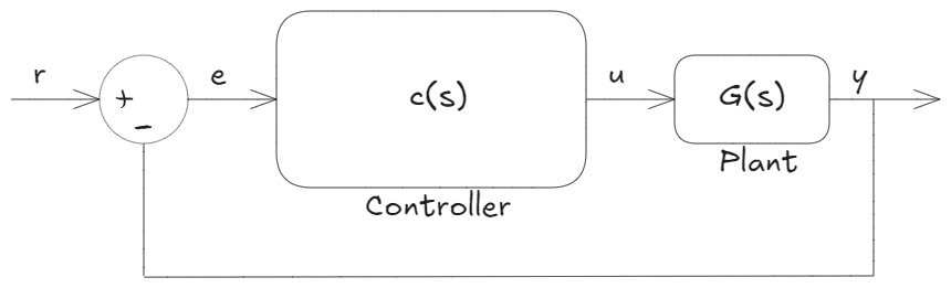
Let's start by understanding the standard feedback control architecture. In this setup:

The plant (the system being controlled) produces an output signal (y)
We take this plant output signal and compare it with our desired input/reference signal (r)
If these two signals don't match, we calculate the difference between them, creating our error signal (e)
The controller examines this error signal and computes a control signal (u)
This control signal is then applied to the plant to adjust its behavior

This feedback loop continuously works to bring the actual output closer to our desired reference.

Starting Simple: Proportional Control

When designing a controller, we should first consider the simplest approach that might work. What's simpler than taking the error and multiplying it by a constant gain value?

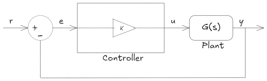
This gives us our first control law:

$$u(t) = K \cdot e(t)$$

This is called proportional control - the "P" in PID. It simply takes the error and multiplies it by a static gain K to compute the control signal. While basic, this approach forms the foundation upon which we'll build our more sophisticated controller.

Expanding to PID Control

PID enhances the basic proportional concept by adding two additional terms, making the control more responsive and accurate:

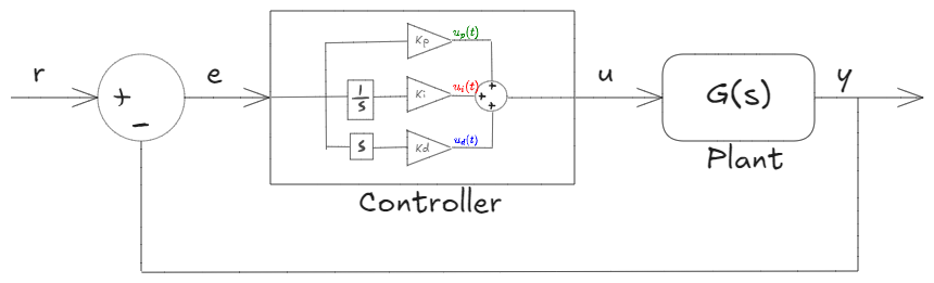
The complete PID control law is:

$$u(t) = K_p \cdot e(t) + K_i \int_{0}^{t} e(\tau) d\tau + K_d \frac{de(t)}{dt}$$

These three components are:

Proportional term: $K_p \cdot e(t)$
Integral term: $K_i \int_{0}^{t} e(\tau) d\tau$
Derivative term: $K_d \frac{de(t)}{dt}$

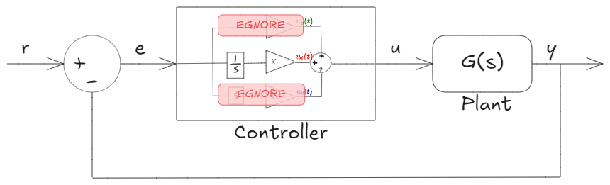
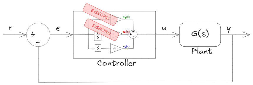
The PID controller's elegance lies in its simplicity. When an error signal reaches the controller, it splits into these three paths. Each path processes the error differently, and the results are summed to produce the final control signal.

Let's examine each component individually to understand its behavior and purpose.

Proportional Control Explained

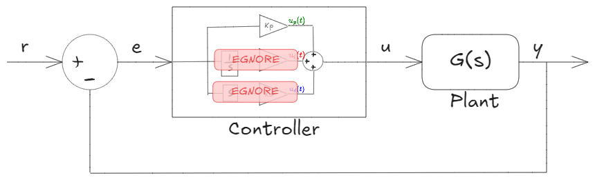
Consider what happens when we have only proportional control:

When the error is zero (meaning our output matches our reference perfectly), the control output is also zero, regardless of what gain value we've chosen. The system is in balance.

Now imagine what happens when we introduce a step change in our reference signal:

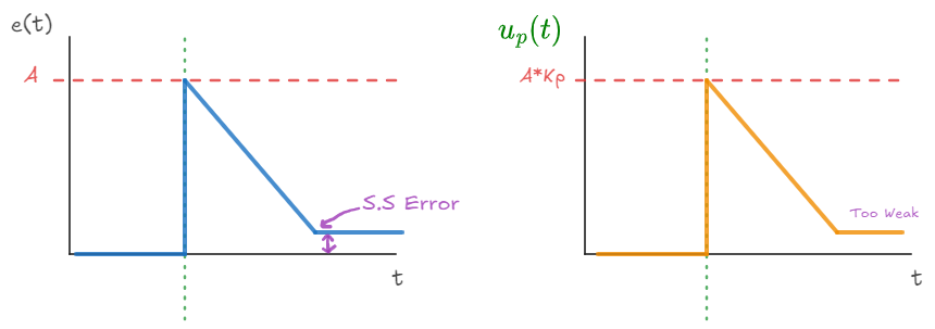
The error jumps up instantly (to point A in our diagram)
The proportional control signal also jumps instantly to $A \times K_p$

This immediate response is the key advantage of proportional control - it reacts instantaneously with no dynamics involved. When the controller "sees" a large error, it applies a large corrective signal to push the system back toward our desired state.

As the system begins to respond, the error decreases. However, as the error gets smaller, the control signal also becomes weaker. This creates an interesting challenge: the control signal gets progressively weaker as we approach our target. At some point, the control signal may become too weak to overcome system friction or other limitations.

For example, if we're controlling a motor to reach a specific angle, each reduction in error leads to a proportional reduction in the voltage applied to the motor. Eventually, we might reach a point where the applied voltage is too small to overcome the motor's internal resistance and friction. This results in a steady-state error - the system stabilizes at a point close to, but not exactly at, our target.

Integral Control Explained

Now let's examine just the integral term: $K_i \int_{0}^{t} e(\tau) d\tau$

This term accumulates the error over time, multiplying the result by the gain factor $K_i$.

When a step change occurs in our system:

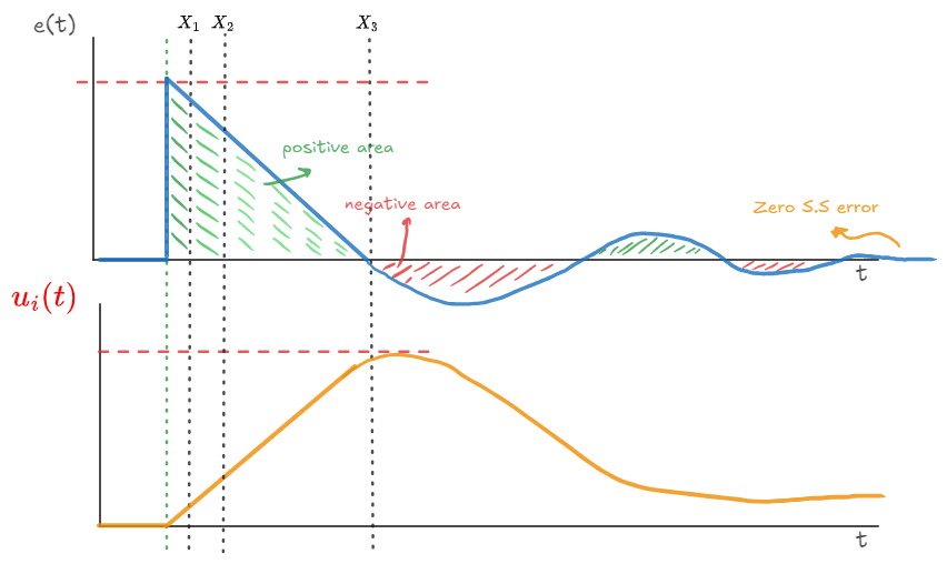
Initially, the integral control signal is small. Even though the error might be large, the controller hasn't had much time to accumulate this error (the area under the curve is small at point X₁).
As time passes (to point X₂), the integral accumulates more area under the error curve, increasing the control signal strength. The controller pushes harder the longer an error persists.
By point X₃, when the error finally reaches zero, the integral has accumulated a significant "history" of error.

What makes integral control interesting is what happens next. Even when the error becomes zero at X₃, the integral control doesn't immediately stop - it continues pushing in the same direction. This causes the system to overshoot the target.

As the error goes negative after overshooting, the integral begins accumulating negative area (shown in red in our diagram). The positive and negative areas eventually balance out, and the system settles at zero error.

The most crucial insight about integral control is that it guarantees zero steady-state error. Here's why:

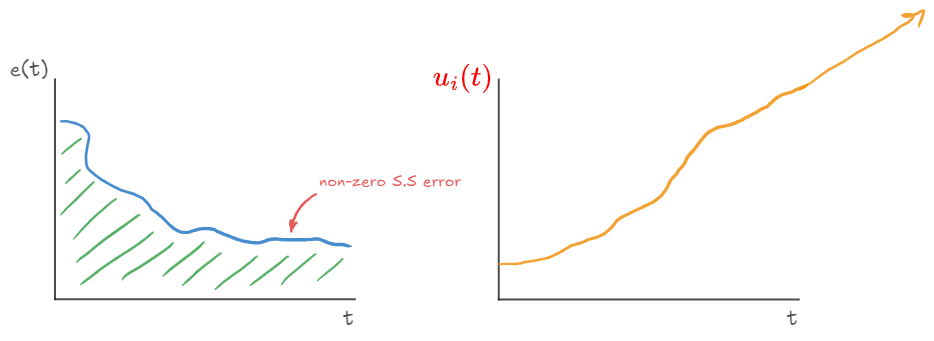
If a non-zero steady-state error were to exist, the integral term would continue accumulating indefinitely. The control signal would grow without bound, eventually becoming strong enough to move the system toward the reference.

This creates a mathematical paradox - with integral control, you simply cannot maintain a non-zero steady-state error indefinitely. The accumulated error would eventually produce a control signal strong enough to overcome any resistance in the system.

This is why integral control is essential for eliminating steady-state errors - it keeps "pushing" until the error becomes zero, no matter how small the error might be.

Derivative Control Explained

The derivative term examines the rate of change of the error: $K_d \frac{de(t)}{dt}$

Unlike the other terms, derivative control cannot operate effectively on its own and is typically combined with proportional control.

When analyzing a step change in our reference:

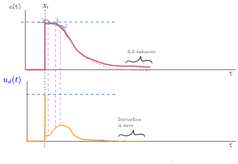
Before the step, the derivative control output is zero since the error is constant (flat error = zero slope)
At the step itself, the slope is theoretically infinite, creating a large spike in the derivative output
As the error begins decreasing, the derivative term responds to the slope at each point

Let's examine this in more detail. At point P1 in our diagram, the slope of the error is small, so the derivative contribution is small. At point P2, the slope is steeper, resulting in a larger derivative control signal. At point P3, where the slope is steepest, the derivative control reaches its maximum strength.

The most important characteristic of derivative control is that it becomes zero at steady state. Once the error stops changing (whether at zero or non-zero steady state), the derivative term contributes nothing to the control signal.

This is why derivative control doesn't help with steady-state error - it only comes into play when the error is actively changing. Its primary purpose is to provide damping during dynamic changes, reducing overshoot and improving stability.

The Complete PID Controller

Now that we understand each term individually, let's see how they work together in a complete PID controller.

The proportional term provides an immediate response proportional to the current error. It forms the backbone of the controller but may result in steady-state error.

The integral term accumulates error over time, ensuring that even small persistent errors will eventually be corrected. This guarantees zero steady-state error but can introduce overshoot and oscillation.

The derivative term responds to the rate of change of error, providing a damping effect that can reduce overshoot and settling time. It helps stabilize the system during rapid changes but contributes nothing at steady state.

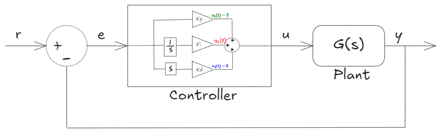
In a perfectly tuned system that has reached zero steady-state error:

The proportional term becomes zero (since the error is zero)
The derivative term becomes zero (since the error is constant)
Only the integral term remains active, providing just enough control signal to maintain the desired output

This interplay between the three components allows PID controllers to achieve excellent performance across a wide range of applications.

Practical Considerations

While the theory above explains the fundamental operation of PID controllers, practical implementation involves careful tuning of the three gain parameters (Kp, Ki, and Kd). The optimal values depend on the specific characteristics of the system being controlled.

Too high a proportional gain can cause instability and oscillation. Too high an integral gain can cause excessive overshoot and slow recovery from disturbances. Too high a derivative gain can amplify noise and make the system overly sensitive to small changes.

The process of finding the right balance between these parameters is called PID tuning, which is both an art and a science in control engineering.

For a practical demonstration of PID control in action, I recommend watching this video starting at the 30:40 mark, which shows how each component affects the behavior of a real system.

Bringing It All Together

PID controllers remain popular because they offer a remarkable balance of simplicity and effectiveness. With just three terms - proportional, integral, and derivative - we can create a controller that responds quickly to changes, eliminates steady-state error, and provides stable operation.

Understanding the individual contributions of each term helps engineers tune PID controllers for optimal performance in specific applications. Whether controlling temperature, position, speed, or countless other variables, the PID algorithm continues to be the cornerstone of modern control systems.

References

Understanding PID Control Systems